Advices for Financial Managers on Mergers and Acquisitions

All financial mangers have to face with followings:

Antitrust Law: Merged companies have to make sure that they are not lessening the competition on any line of business or they are not imposing a monopoly on the market.

The Form of Financing: There are two types of mergers that are distinguished by how the merger is financed. Each has certain implications for the companies involved and for investors:

• Purchase Mergers - As the name suggests, this kind of merger occurs when one company purchases another. The purchase is made with cash or through the issue of some kind of debt instrument; the sale is taxable.
  Acquiring companies often prefer this type of merger because it can provide them with a tax benefit. Acquired assets can be written-up to the actual purchase price, and the difference between the book value and the purchase price of the assets can depreciate annually, reducing taxes payable by the acquiring company.
• Consolidation Mergers - With this merger, a brand new company is formed and both companies are bought and combined under the new entity.

See this for more detail.

Merger Accounting: A method of accounting for a business combination. It may only be used when a business combination falls within the definition of a merger defined in associated Laws. A business combination meets the definition of a merger under the Companies Act only if it involves the exchange of equity shares for equity shares such that a stake of more than 90% is acquired and generally accepted accounting principles permit the use of merger accounting.

Tax Considerations: When making an acquisition, disposing of a non-core business or going through a merger, companies need to manage tax risk and ensure future net cash flows are optimised.

Incentives for Mergers and Acquisitions

Followings are incentives for financial managers for mergers and acquisitions:

Economies of Scale: Economies of scale characterizes a production process in which an increase in the number of units produced causes a decrease in the average cost of each unit. Mergers also translate into improved purchasing power to buy equipment or office supplies - when placing larger orders, companies have a greater ability to negotiate prices with their suppliers.

Economies of Vertical Integration: Achieving lower operating costs by bringing the entire production chain within the firm rather than contracting through the marketplace. The most common way is merging with a company at a different stage in the production process, for instance, a car maker merging with a car retailer or a parts supplier.Companies buy companies to reach new markets and grow revenues and earnings. A merge may expand two companies' marketing and distribution, giving them new sales opportunities. A merger can also improve a company's standing in the investment community: bigger firms often have an easier time raising capital than smaller ones.

Complementary Resources: Most likely to end up with acquisitions when a big firm sees an opportunity in the small one which has technology, competitiveness talented team etc. If small company has insufficient resources to finance its own projects two companies may prefer to merge and complete each other's needs.

Surplus Funds: It is about spending excess of earnings to fund mergers and acquisitions instead of investing it on new projects of paying out dividends or buying back stocks.

Eliminating Inefficiencies: As every employee knows, mergers tend to mean job losses. Consider all the money saved from reducing the number of staff members from accounting, marketing and other departments. Job cuts will also include the former CEO, who typically leaves with a compensation package.

Industry Consolidation: If market has too many entities and each one is competing to gain more slice from it, merging can be seen as a good way to consolidate to gain more competitiveness.

Adjusted Present Value (APV)

There is no argument that WACC is the most widely used method to asses the overall cost of capital to judge business whether it is profitable or not. However WACC has also limitations and its calculations are bound to equity and debt financing and their calculated ratios. When projects have side effects which have other contributions on cost of capital, the APV model is more handy.

Adjusted present value (APV) is similar to NPV. The difference is that is uses the cost of equity as the discount rate (rather than WACC). This is because an assumption is made as the company is all financed through equity and leverage is zero at start. Then separate adjustments are made for all other side effects (e.g. the tax advantages of debt).

As usual with DCF models of this sort, the calculation of adjusted present value is straightforward but tedious.

The Mechanics of APV Valuation

The first step in calculating an APV is to calculate a base NPV using the cost of equity as the discount rate. This may be the same as the company's cost of equity. In some cases it may be necessary to recalculate it by estimating a beta and using CAPM. This is most likely when assessing a project or business that is very different from a company's core business.

Once the base NPV has been calculated, the next step is to calculate the NPV of each set of cash flows that results from financing. The most obvious of these are the tax effects of using debt rather than equity. These can be discounted either at the cost of debt or at a higher rate that reflects uncertainties about the tax effects (e.g. future tax rates, whether the company as a whole will be profitable and paying tax). The NPV of the tax effects is then added to the base NPV.

If there are other effects of financing, then these are also added or subtracted, and the end result is the APV.

In brief,  we estimate the value of the firm in three steps. We begin by estimating the value of the firm with no leverage. We then consider the present value of the interest tax savings generated by borrowing a given amount of money. Finally, we evaluate the effect of borrowing the amount on the probability that the firm will go bankrupt, and the expected cost of bankruptcy.

Cost of Capital versus APV Valuation

In the cost of capital approach, the effects of leverage show up in the cost of capital, with the tax benefit incorporated in the after-tax cost of debt and the bankruptcy costs in both the levered beta and the pre-tax cost of debt. Will the two approaches yield the same value? Not necessarily. The first reason for the differences is that the models consider bankruptcy costs very differently, with the adjusted present value approach providing more flexibility in allowing you to consider indirect bankruptcy costs. To the extent that these costs do not show up or show up inadequately in the pre-tax cost of debt, the APV approach will yield a more conservative estimate of value. The second reason is that the APV approach considers the tax benefit from a dollar debt value, usually based upon existing debt. The cost of capital approach estimates the tax benefit from a debt ratio that may require the firm to borrow increasing amounts in the future. For instance, assuming a market debt to capital ratio of 30% in perpetuity for a growing firm will require it to borrow more in the future and the tax benefit from expected future borrowings is incorporated into value today.

There are many who believe that adjusted present value is a more flexible way of approaching valuation than traditional discounted cash flow models. This may be true in a generic sense, but APV valuation in practice has significant flaws. The first and most important is that most practitioners who use the adjusted present value model ignore expected bankruptcy costs. Adding the tax benefits to unlevered firm value to get to the levered firm value makes debt seem like an unmixed blessing. Firm value will be overstated, especially at very high debt ratios, where the cost of bankruptcy is clearly not zero and, in some instances, the cost of bankruptcy is higher than the tax benefit of debt.

T tests on Regression Equations

One of the advantages of the regression equations is that we can run t tests on the individual regression coefficients. t tests help us to determine whether the coefficient is significant or not for the associated independent variable. Through the t tests we can understand whether a particular independent variable has on effect on the output, holding the other independent variables constant.

We start the t tests by making an assumption that the coefficient is equal to zero. So that we can measure how much this coefficient is different from zero, regardless of the sign. (Difference can be negative or positive). If test result yields lower than the critical value given in the t-distributions table, we can come to conclusion that this particular coefficient is insignificant for the output; otherwise it is accepted as significant. Therefore our hypotheses can be written as:

H0 : Bi = 0,     H1 : Bi ≠ 0       

where H0 (null hypothesis) is for assuming Bi as zero; whereas H1 (alternative hypothesis) is for assuming Bi as different from zero. Since we don’t care the sign of the difference this is a two-tailed t-test. and t is defined as:

         

 

Once we calculate all t values for each B value in a regression equation, we find the critical t value from the table and then decide whether they fall under this critical value or not. Values fall under critical value is accepted as insignificant and others are significant.

Regression Model for Exposure Estimation

Adler and Dumas defined exposure elasticity as the changes in the market value of a firm with respect to the change in exchange using following time series regression:

Rit = b0i + b1iRst + eit,     t = 1, …,T,        (1)

where Rit is the stock return for firm i, Rst is the percentage change in an exchange rate variable, measured as home currency price of foreign currency. Therefore a positive value for Rst indicates a home currency depreciation. bit is the elasticity of firm to the changes in exchange rate. This elasticity indicates the firm’s average exposure over the estimation period. b0i reflects common stock value, when expected rate of change in the exchange rate is constant over time
In order to control macroeconomic influences on returns, most recent empirical studies include market return in the model. This market return parameter not just helps to control macroeconomic influences but also reduces residual variances of the equation (1). Therefore most common form of regression equation for exchange rate exposure is described as follows:

Rit = b0i + b1iRst + b1iRmt + eit,    i =1, … , N;       t = 1, … ,T        (2)

where Rmt is the rate of return on market index, N is the number of cross sections, T is the length of the time series for each cross section.

Whether they are simple or multiple regressions each coefficient tells us what relation that input variable has with output variable (where all other input variables are held constant). In linear models in order to get the real elasticity one must multiply the slop coefficient by its input variable and then divide by the output.

The relation between inputs and output may not always be linear. We can take Cobb-Douglas production function as an example, which is widely used in empirical researches. It is defined as:

       (3)

where b1 is a constant and can be thought a scaling factor and b2 and b3 are coefficients. Although this equation is non-linear, it can be transformed to linear by taking natural logarithms of both sides.

ln yi = ln b1 + b2 lnx2i + b3 lnx3i + ui         (4)

The equation (4) is linear in the parameters but non linear in the variables. In this equation the slope is no more constant and it changes according to input and output variables. One big advantage of this equation is that the coefficients gives us partial elasticities. E.g. b2 is the partial elasticity of output yi with respect to the x2i, holding x3i constant.

Strengths and Weaknesses of Ratio Analysis

Ratio analysis can reveal most of the information about the company when it is used effectively. An analyst must be aware of the strengths and weakness of this method for correct assessing these values. Following explains the strengths and weaknesses of this method.

Strengths

Ratio analysis can be very helpful when the values are compared against previous years, other companies, industry averages. These comparisons help analyst to identify company’s strengths and weaknesses and evaluate its financial position and also foresee the risks that may emerge in the future.

Using ratios a financial analyst can implement plans to improve profitability, liquidity, gearing problems and market value of the business. Although ratios report on past performances, they can be used for predictive purposes to catch potential problems. It is possible to verdict if the company has enough liquidity to pay its future debts or even tell whether its shareholders will be happy.

Weaknesses

Not all financial ratios can be compared. There are several points that analyst must take into account. When two companies' financial data is compared, the ratios must reflect comparable price levels and these values must be evaluated using same accounting methods and valuation bases. Also, such comparisons should be limited to companies engaged in similar business activities. If the financial policies differ, this must be recognized while evaluating of comparative reports. For example one company leases its properties while the other purchases such items; one company finances its business using long-term borrowing while the other provide its fund by shareholders and reserves. In these cases, ratios can not be compared.

Comparing ratios with past data of the same company (trend analysis) can indicate the performance over years and highlight points that need for action, however it will not be enough to tell much about the company’s status among competitors. For more informative analysis, ratios should be compared with two or more companies in similar line of business (cross-sectional analysis). More reasonable method would be comparing ratios to industry averages, which are developed by statistical services and trade associations.

There is no single or correct value for a ratio. The value may be too low or to high against to reference value. Ratios may mislead when they are not combined with company’s management and economic circumstances. Analyst must consider company’s products, competitors and also the company’s vision for the future.

In the trend analysis although 2 years comparison can give the idea about the performance of the company, it is best to use three to five years of ratios to have broader view of performance. Seasonal variations also must be looked at attentively in trend analysis.

Another point about ratios is that they could be evaluated with different methods and they are dependent on the perspective of the analyst. Therefore it is not always possible to define “good” and bad for the values.

Analysing Company with Financial Ratios

Profitability

Profitability is "the ability for a company to earn satisfactory profit so that the investors and shareholders will continue to provide capital to it." For this reason profitability ratios are much observed by the investors and by the shareholders.

One of the principal ratios related to profitability is profit margin. Two major profit margins widely known are: "net profit margin" (NPM) and "gross profit margin" (GPM). Both of these margins are calculated by dividing income (profit) by turnover (sales). In the Gross Profit Margin, income is calculated before operating expenses, interest and tax, whereas in the net profit margin all these expenses are taken out from income.

NPM is the function of the sale price of the product and efficiency of sale cost. For the companies, which are selling a unique product to a captive market may be able to charge a premium price and thus generate greater NPM. A company, which is selling a generic product in a highly competitive market, will have a low NPM. Therefore, it must be a very efficient company.

Another principal ratio is return of capital employed (ROCE). It is the amount of profit as a percentage of capital employed. This ratio is the most important measure of the business performance of a company, since it assess how much the capital invested has earned during a period. The fall of ROCE is not a good sign for an investor who is considering investment on this company.

Liquidity

Being a profitable company does not mean that it can pay its creditors, expenses, loans when they become due. Companies' ability to meet its requirements for both expected and unexpected cash demand is defined as liquidity. All businesses need some liquidity to operate. If company has too little liquidity, it may result in bankruptcy in case of urgent money demands. However, having more liquidity than what the business needs could take the profit away, since they are low returning investments.

There are two main ratios as liquidity indicators: "current ratio" and "quick ratio". Both ratios are defined as the ratio of current assets to current liabilities, whereas, in the quick ratio, stocks are excluded from the current assets. These ratios are observed by the suppliers and providers to assess the ability of the business to pay its dues.

Recommended values for current ratio is 2:1, meaning business should have twice the current assets of its current liabilities and for quick ratio is 1:1. However, the real values may be much different from those suggested values, since different businesses operate in different ways. Current ratio is expected to be a bit higher for smaller companies, since they may have to cover unforeseen cash demands from current assets. It is also possible to figure out how much stock is used by looking at the differences between current and quick ratios.

Gearing (Debt Management)

Gearing is a method of comparing how much of the long-term capital of a business is provided by equity (ordinary shares and reserves) and how much is provided by prior charge capital (preference shares and loans). When a company makes profit, first the fixed claims of preference shareholders and creditors are met. Then, rest of the profit is shared by ordinary shareholders. If this is a profitable company, ordinary shareholders become main beneficiaries, if it is not, then they may receive a little or nothing at all.

A business with larger prior charge capital to equity capital is said to be highly geared. High level of gear carries a risk and represents legal obligations to pay dividends periodically. Failure to make these payments can result in bankruptcy.

Debt ratio is used to measure the gearing level of the business and it is calculated as the prior charge capital divided by total assets.

Investor’s Ratios (Market Value)

These ratios reflect relationship between the amount of return and the value of investment provided by ordinary shareholders.

One principal ratio is earnings per share (EPS) and it measures the profit earned per share. It is calculated by ratio of profit (distributed or retained) to the number of ordinary shares. The higher EPS attract more investors and more equity to business.

In order to make more comprehensive analysis we might need additional investor’s ratios like dividend yield and price earning ratios. Dividend yield ratio would give information to shareholders how much dividend is earned from the market value of the shares. And price earning ratio is calculated by dividing the company's share price by EPS. This gives an indication of how many times an investor is paying for a company's share verse a company's earnings. Higher P/E ratios are often seemed as an indication for a company that is growing faster than average and investors believe that the company's earnings will be higher in the future.

Apart from the additional ratios, an analyst may request more than 2 years of ratios to see wider perspective of the company performance. However having many years of ratio values and different types of ratios do not tell about the size of the business, other financial statements must be investigated for full analysis.

Binomial Option Pricing Model

Another options valuation model developed by Cox, et al, in 1979.  The binomial option pricing model uses an iterative procedure, allowing for the specification of nodes, or points in time, during the time span between the valuation date and the option's expiration date.

The model  makes following assumptions:

• No price changes,
• No arbitrage,
• Efficient market, short duration of options.

Under these assumptions, it is able to provide a mathematical valuation of the option via a binomial lattice (tree), at each point in time specified. A simplified example of a binomial tree might look something like this:

 

Each node in the lattice, represents a possible price of the underlying, at a particular point in time.

The valuation process is iterative, starting at each final node, and then working backwards through the tree to the first node (valuation date), where the calculated result is the value of the option.

Option valuation using this method is, as described, a three step process:

1. Price tree generation
2. Calculation of option value at each final node
3. Progressive calculation of option value at each earlier node; the value at the first node is the value of the option.

The tree of prices is produced by working forward from valuation date to expiration

At each step, it is assumed that the underlying instrument will move up or down by a specific factor (u or d) per step of the tree (where, by definition, and ). So, if S is the current price, then in the next period the price will either be or .

The up and down factors are calculated using the underlying volatility, σ and the time duration of a step, t, measured in years (using the day count convention of the underlying instrument). From the condition that the variance of the log of the price is σ²t, we have:

Due to its simple and iterative structure, the model presents certain unique advantages. For example, since it provides a stream of valuations for a derivative for each node in a span of time, it is useful for valuing derivatives such as American options which allow the owner to exercise the option at any point in time until expiration (unlike European options which are exercisable only at expiration). The model is also somewhat simple mathematically when compared to counterparts such as the Black-Scholes model, and is therefore relatively easy to build and implement with a computer spreadsheet.

Although slower than the Black-Scholes model, it is considered more accurate, particularly for longer-dated options, and options on securities with dividend payments. For these reasons, various versions of the binomial model are widely used by practitioners in the options markets.

1. http://www.investopedia.com/terms/b/binomialoptionpricing.asp
2. http://en.wikipedia.org/wiki/Binomial_options_model

Tax Types & Descriptions

HM Revenue & Customs collects tax to pay for public services. Each year the Chancellor's Budget sets out how much it'll cost to provide these services and how much tax is needed to pay for them. Key taxes that individuals may have to pay include: Income Tax, Capital Gains Tax, Inheritance Tax, Stamp Duty, Value Added Tax and certain other duties.

Personal Taxes

Income Tax

Income Tax is paid on:

• your wages if you're employed
• the profits from your business if you're self-employed
• your State Pension and any private pensions
• some benefits like Jobseeker's Allowance, Carer's Allowance and Incapacity Benefit

Capital Gains Tax

CGT is a tax on capital 'gains'. If when you sell or give away an asset it has increased in value, you may be taxable on the 'gain' (profit). This doesn't apply when you sell personal belongings worth £6,000 or less or, in most cases, your main home.

You may have to pay CGT if, for example, you:

• sell, give away, exchange or otherwise dispose of (cease to own) an asset or part of an asset
• receive money from an asset - for example compensation for a damaged asset

You don't have to pay CGT on:

• your car
• your main home - provided certain conditions are met
• ISAs or PEPs
• UK Government gilts (bonds)
• personal belongings worth £6,000 or less when you sell them
• betting, lottery or pools winnings
• money which forms part of your income for income tax purposes

Inheritance Tax

Inheritance Tax is the tax that is paid on your 'estate'. Broadly speaking this is everything you own at the time of your death, less what you owe. It's also sometimes payable on assets you may have given away during your lifetime. Assets include things like property, possessions, money and investments.

Stamp Duty

Stamp Duty is the tax you pay when you buy property or shares. You pay 'Stamp Duty Land Tax' when you buy property and either 'Stamp Duty' or 'Stamp Duty Reserve Tax' when you buy shares.

You pay Stamp Duty Land Tax on property like houses, flats, other buildings and land. If the purchase price is £125,000 or less you don't pay any Stamp Duty Land Tax at all. If it's more than £125,000, you pay between one and four per cent of the whole purchase price.

Value Added Tax

VAT is a tax that you pay when you buy goods and services in the European Union (EU), including the United Kingdom. Where VAT is payable it's normally included in the price of the goods or service you buy. Some goods don't attract VAT.

Each EU country has its own rates of VAT. In the UK there are three rates.

Standard rate: You pay VAT on most goods and services in the UK at the standard rate, currently 17.5 per cent.

Reduced rate: In some cases, for example childrens car seats and domestic fuel or power, you pay a reduced rate of five per cent.

Zero rate: There are some goods on which you don't pay any VAT, like:

• food
• books, newspapers and magazines
• children's clothes
• special exempt items - for example equipment for disabled people

Business Taxes (Corporate Taxes)

Corporate taxes are imposed on domestic and foreign corporations that are engaged in business activities, employ capital, own or lease property, or maintain an office. In UK Corporate tax is not payable by the self-employed but does apply to the following organisations, even if they are not limited companies:

• members' clubs, societies and associations
• trade associations
• housing associations
• groups of individuals carrying on a business but not as a partnership, eg co-operatives

Corporation tax is charged on the profits made by companies, public corporations and unincorporated associations. The tax is charged on the profits made in each accounting period, ie the period over which the company draws up its accounts. The rates of tax are set for the financial year April to March; where an accounting period straddles 31 March the profits are apportioned between the two financial years on a time basis.

Deductions are allowed from a company's total profits for any charges (interest and other payments) it pays and, in the case of an investment company, its management expenses. From April 1996, new "loan relationship" rules have been in force for the treatment of interest and similar payments. A deduction against the tax liability is allowed for income tax deducted at source from interest received (to the extent that it is not used to cover income tax the company itself deducts on interest payments it makes). Double taxation relief for foreign tax is allowed as a deduction against the tax charged on profits.

Agency Costs

Shareholders, bondholders, employees, customers, management, suppliers, etc. All of these are called stakeholders. Much debate as to which group deserves most attention. Although there is widespread agreement that shareholders are the most important group of stakeholders, there are still many conflicts between the various stakeholder groups. Bond is a debt security, in which the authorized issuer owes the holders a debt and is obliged to repay the principal and interest (the coupon) at a later date, termed maturity. Bonds and stocks are both securities, but the difference is that stock holders own a part of the issuing company (have an equity stake), whereas bond holders are in essence lenders to the issuer

An agency cost is an economic concept on the cost incurred by an organization that is associated with problems such as divergent management-shareholder objectives and information asymmetry.

The information asymmetry that exists between shareholders and the Chief Executive Officer is generally considered to be a classic example of a principal-agent problem. The agent (the manager) is working on behalf of the principal (the shareholders), who does not observe the actions of the agent. This information asymmetry causes the agency problems of moral hazard and adverse selection.

According to Ross and Westerfield when a firm has debt, conflicts of interest arise between shareholders and bondholders. Because of this, shareholders are tempted to pursue selfish strategies, imposing agency costs on the firm. These strategies are costly, because they lower the market value of the whole firm.

Followings are examples to agency costs that a firm might have to incur:

• profit-sharing bonuses
• contingency fees
• sales commissions
• merit raises
• executive stock options
• and various other contractually specified methods of setting the amount of the agent's financial compensation in proportion to measurable results

References:

1. http://www.auburn.edu/~johnspm/gloss/agency_problem

Market Timing Hypothesis

The market timing hypothesis was first introduced by Wurgler and Baker in the year of 2004. It states that firms look for the cheaper type of financing regardless of their current levels of internal resources, debt and equity. This theory has been suggested as an alternative to the widely known theories like trade off theory and pecking order theory and tries to explain the incentives for a financial manager to find optimum capital structure.

The market timing hypothesis says that the first order determinant of the capital structure of a corporation represents the proportional mis-pricing of the debt and equity portions when the firm requires funds for investments. In other words firms usually do not care whether the financing is done with equity or debt. The firms and corporations select the most suitable form of financing at the time of investment.

Theory itself does not give any reason why mis-pricing exists but assumes that the mis-pricing exists in the market. The theory also gives an account on the firm's behavior with the assumption that the firms are able in detecting the mis-pricing more efficiently than the markets.
The empirical evidence, whether this hypothesis holds in the real world is mixed. The market timing typically refers to the decision of the buying or selling of the financial assets such as stocks while trying to predict the price movements of the future market. The prediction is usually based the market outlook or on the economic conditions coming out from the fundamental or technical analysis of the market.

References:

1. http://finance.mapsofworld.com/corporate-finance/hybrid-financing/marketing-timing-hypothesis.html
2. Market timing hypothesis - Wikipedia, the free encyclopedia

Internal Rate of Return (IRR)

Mathematically the IRR is defined as any discount rate that results in a net present value of zero of a series of cash flows.

If the internal rate of return is less than the cost of borrowing used to fund your project, the project will clearly be a money-loser. However, usually a business owner will insist that in order to be acceptable, a project must be expected to earn an IRR that is at least several percentage points higher than the cost of borrowing, to compensate the company for its risk, time, and trouble associated with the project.

 

C_t = cash flow in period t, and N = the number of periods.

Example:

Assume that a company has following cash flows for 5 periods ahead.

Year	0	1	2	3	4
Cash Flow	-100	+30	+35	+40	+45

The IRR of an investment is the interest rate that will give it a net present value of zero.

Oddly, IRR is calculated trough trial and error method. For the example above, the IRR is 17.09

IRR analysis is generally used to evaluate the project's cash flows, rather than the income from the project that would be shown on an income statement (also known as the profit and loss statement). Why? Because income on a P&L reflects depreciation, but depreciation is not an out-of-pocket expense. For instance, if revenue of $10,000 is reduced to $7,000 of income because of a $3,000 depreciation deduction, you still have the use of the full $10,000. So the cash flow figure of $10,000 is usually the more instructive one to look at. However, if you are very concerned about the appearance of your income statement (for example, if you anticipate putting the business up for sale or seeking major financing in the future, or if you're under stockholder pressure for increased income) you may decide that the income figure is more appropriate to use.

References:

1. http://www.toolkit.com/small_business_guide/sbg.aspx?nid=P06_6550
2. http://moneyterms.co.uk/irr/
3. http://en.wikipedia.org/wiki/Internal_rate_of_return
   

Working capital

Working capital is the difference between current assets and current liabilities and simply calculated by

Working capital  = current assets  - current liabilities

Following a simple break down of what current assets and liabilities might be.

Analysis of working capital is especially important for the firms that work on inventories rather than fixed assets or people resources. Most common example is the retailers that hold huge amount of inventories. Inventory forms major part of their assets and seeing their value is important to asses their current financial status in the market.

There are mainly two important implications of working capital:

1. If a company's current assets do not exceed its current liabilities, then it may run into trouble paying back creditors in the short term. The worst-case scenario is bankruptcy. A decline in working capital ratio in the long term could be a red flag that requires further analysis. For example, it could be that the company's sales volumes are falling.
2. Working capital also gives investors an idea of the company's underlying operational efficiency. Money that is tied up in inventory or money that customers still owe to the company cannot be used to pay off any of the company's obligations. So, if a company is not operating in the most efficient manner, it will show up as an increase in the working capital. The working capital values can be compared with older terms to see if there is any slowness in the collection of money. That slowness might be an another indication of problem in the company's operations.

The widely observed indicator to see whether working capital is used efficiently is Cash Conversion Cycle.

Cash Conversion Cycle

The cash conversion cycle is the number of days between paying for inventories and receiving cash from selling these inventories or any goods made from that inventories. The cash conversion cycle is a measure of working capital efficiency, often giving valuable clues about the underlying health of a business. The higher the number, the longer a firm's money is tied up in business operations and unavailable for other activities such as investing.

Since a company uses its cash to buy inventory but does not collect cash until the inventory is sold, the days inventory outstanding (DIO) (the number of days that inventories are kept unsold) and the days sales outstanding (DSO) (the number of days that goods stay for sale) are summed up. However, days payable outstanding (DPO) which essentially represent loans from vendors to the company is subtracted as relief for working capital needs. The cash conversion cycle is given by the following formula:

CCC = DSO+DIO-DPO

• DIO: days inventory outstanding.
• DSO: days sales outstanding.
• DPO: days payable outstanding.

References:

1.  http://www.schaeffersresearch.com/schaeffersu/advanced/financialstatements/financialstatements6.aspx

2. http://en.wikipedia.org/wiki/Cash_conversion_cycle

3. http://www.investopedia.com/terms/w/workingcapital.asp

Capital Management Decisions

Following beautifully written text has been taken from here. So if you wonder where the origin is please refer to there.

... Decisions can be divided into long-term and short-term decisions and techniques. Capital investment decisions are long-term choices about which projects receive investment, whether to finance that investment with equity or debt, and when or whether to pay dividends to shareholders. On the other hand, the short term decisions can be grouped under the heading Working capital management. This subject deals with the short-term balance of current assets and current liabilities; the focus here is on managing cash, inventories, and short-term borrowing and lending (such as the terms on credit extended to customers).

Capital investment decisions

Capital investment decisions are long-term corporate finance decisions relating to fixed assets and capital structure. Decisions are based on several inter-related criteria. Corporate management seeks to maximize the value of the firm by investing in projects which yield a positive net present value when valued using an appropriate discount rate. These projects must also be financed appropriately. If no such opportunities exist, maximizing shareholder value dictates that management return excess cash to shareholders. Capital investment decisions thus comprise an investment decision, a financing decision, and a dividend decision.

Project valuation

In general, each project's value will be estimated using a discounted cash flow (DCF) valuation, and the opportunity with the highest value, as measured by the resultant net present value (NPV) will be selected. This requires estimating the size and timing of all of the incremental cash flows resulting from the project. These future cash flows are then discounted to determine their present value. These present values are then summed, and this sum net of the initial investment outlay is the NPV.

The NPV is greatly influenced by the discount rate. Thus selecting the proper discount rate—the project "hurdle rate"—is critical to making the right decision. The hurdle rate is the minimum acceptable return on an investment—i.e. the project appropriate discount rate. The hurdle rate should reflect the riskiness of the investment, typically measured by volatility of cash flows, and must take into account the financing mix. Managers use models such as the CAPM or the APT to estimate a discount rate appropriate for a particular project, and use the weighted average cost of capital (WACC) to reflect the financing mix selected. (A common error in choosing a discount rate for a project is to apply a WACC that applies to the entire firm. Such an approach may not be appropriate where the risk of a particular project differs markedly from that of the firm's existing portfolio of assets.)

In conjunction with NPV, there are several other measures used as (secondary) selection criteria in corporate finance. These are visible from the DCF and include payback period, IRR, Modified IRR, equivalent annuity, capital efficiency, and ROI.

The financing decision

Achieving the goals of corporate finance requires that any corporate investment be financed appropriately. As above, since both hurdle rate and cash flows (and hence the riskiness of the firm) will be affected, the financing mix can impact the valuation. Management must therefore identify the "optimal mix" of financing—the capital structure that results in maximum value.

The sources of financing will, generically, comprise some combination of debt and equity. Financing a project through debt results in a liability that must be serviced—and hence there are cash flow implications regardless of the project's success. Equity financing is less risky in the sense of cash flow commitments, but results in a dilution of ownership and earnings. The cost of equity is also typically higher than the cost of debt (see CAPM and WACC), and so equity financing may result in an increased hurdle rate which may offset any reduction in cash flow risk.

Management must also attempt to match the financing mix to the asset being financed as closely as possible, in terms of both timing and cash flows.

One of the main theories of how firms make their financing decisions is the Pecking Order Theory, which suggests that firms avoid external financing while they have internal financing available and avoid new equity financing while they can engage in new debt financing at reasonably low interest rates. Another major theory is the Trade-Off Theory in which firms are assumed to trade-off the Tax Benefits of debt with the Bankruptcy Costs of debt when making their decisions. One last theory about this decision is the Market timing hypothesis which states that firms look for the cheaper type of financing regardless of their current levels of internal resources, debt and equity.

The dividend decision

In general, management must decide whether to invest in additional projects, reinvest in existing operations, or return free cash as dividends to shareholders. The dividend is calculated mainly on the basis of the company's unappropriated profit and its business prospects for the coming year. If there are no NPV positive opportunities, i.e. where returns exceed the hurdle rate, then management must return excess cash to investors. These free cash flows comprise cash remaining after all business expenses have been met.

This is the general case, however there are exceptions. For example, investors in a "Growth stock", expect that the company will, almost by definition, retain earnings so as to fund growth internally. In other cases, even though an opportunity is currently NPV negative, management may consider “investment flexibility” / potential payoffs and decide to retain cash flows.

Management must also decide on the form of the distribution, generally as cash dividends or via a share buyback. There are various considerations: where shareholders pay tax on dividends, companies may elect to retain earnings, or to perform a stock buyback, in both cases increasing the value of shares outstanding; some companies will pay "dividends" from stock rather than in cash. Today it is generally accepted that dividend policy is value neutral (see Modigliani-Miller theorem).

Working capital management

Decisions relating to working capital and short term financing are referred to as working capital management. These involve managing the relationship between a firm's short-term assets and its short-term liabilities. The goal of Working capital management is to ensure that the firm is able to continue its operations and that it has sufficient cash flow to satisfy both maturing short-term debt and upcoming operational expenses.

Decision criteria

By definition, Working capital management entails short term decisions - generally, relating to the next one year period - which are "reversible". These decisions are therefore not taken on the same basis as Capital Investment Decisions (NPV or related, as above) rather they will be based on cash flows and / or profitability.

• One measure of cash flow is provided by the cash conversion cycle - the net number of days from the outlay of cash for raw material to receiving payment from the customer. As a management tool, this metric makes explicit the inter-relatedness of decisions relating to inventories, accounts receivable and payable, and cash. Because this number effectively corresponds to the time that the firm's cash is tied up in operations and unavailable for other activities, management generally aims at a low net count.

• In this context, the most useful measure of profitability is Return on capital (ROC). The result is shown as a percentage, determined by dividing relevant income for the 12 months by capital employed; Return on equity (ROE) shows this result for the firm's shareholders. Firm value is enhanced when, and if, the return on capital, which results from working capital management, exceeds the cost of capital, which results from capital investment decisions as above. ROC measures are therefore useful as a management tool, in that they link short-term policy with long-term decision making.

References:

1. http://en.wikipedia.org/wiki/Corporate_finance

Arbitrage Pricing Theory (APT)

This is one of which the two prevailing theories that try to explain valuation of assets. The other is Capital Asset Pricing Model which can be considered the special case of APT. In this theory it is believed that the factors that have an effect on the value of particular asset form the equation that gives the expected return of this asset. The formula is expressed as follows:

r = r_f + β₁f₁ + β₂f₂ + β₃f₃ + ...

• r expected return
• r_f risk free rate
• f factor
• β measure of the relationship between the security price and that factor.

The model is based on the idea that if any divergence occurs at the price of a particular asset, the arbitrage process brings its value back into line.

The difference between CAPM and arbitrage pricing theory is that CAPM has a single non-company factor and a single beta, whereas arbitrage pricing theory divides them into different factors. Each factor has a separate beta. The beta of each factor is the sensitivity of the price of the security to that factor.

APT directly relates the price of the security to the fundamental factors driving it. APT does not suggests what type of factors drive the valuation of that security. Therefore these factors need to be worked out empirically. The most obvious factors are economic growth and interest rates. For companies in some sectors other factors are obviously relevant as well - such as consumer spending for retailers.

The value of Betas are calculated through linear regression analysis of historical security returns on the factor in question. The number and the nature of these factors, hence betas, are likely to change over time along with economic conditions.

Opportunity Cost

If an investor has alternative projects but has a limited resources one or some of them have to preferred over the others. In such cases the cost of difference between preferred  investment(s) and the one(s) that have been given up is called opportunity cost.

For example you invest in a stock and it returns 4% over the year. In placing your money in the stock, you gave up the opportunity of another investment - for example, a risk-free government bond yielding 6%. In this case, your opportunity cost is 2% (6% - 4%).

Opportunity cost can be applied on any decision that has alternatives put this in another way; any decision that involves a choice between two or more options has an opportunity cost. Following example is most common one, given to explain opportunity cost in areas other than finance.

If you are working and having a steady stream of salary and decide to go to a university by having a break in your career, then you must give up your earnings for a certain period and pay your study fees. The rational behind such a decision can be the offset of higher salary you are projecting by having a better degree.

Consider the case of an MBA student who pays £16,000 per year in tuition and fees at a university. For a two-year program, the cost of tuition and fees would be £32,000. This is the monetary cost of the education. However, when making the decision to go back to school, opportunity cost, which includes the income that the student would have earned if the alternative decision of remaining in his or her job had been made. If the student had been earning £35,000 per year £70,000 in salary would be given up Adding this amount to the educational chargers results in a cost of $102,000 for such a degree.

As another example, if a shipwrecked sailor on a desert island is capable of catching 10 fish or harvesting 5 coconuts in one day, then the opportunity cost of producing one coconut is two fish (10 fish / 5 coconuts). Note that this simple example assumes that the production possibility frontier between fish and coconuts is linear.

Relative Price

Opportunity cost is expressed in relative price, that is, the price of one choice relative to the price of another.

For example, if milk costs $4 per gallon and bread costs $2 per loaf, then the relative price of milk is 2 loaves of bread. If a consumer goes to the grocery store with only $4 and buys a gallon of milk with it, then one can say that the opportunity cost of that gallon of milk was 2 loaves of bread (assuming that bread was the next best alternative).

In many cases, the relative price provides better insight into the real cost of a good than does the monetary price.

Applications of Opportunity Cost

The concept of opportunity cost has a wide range of applications including:

• Consumer choice
• Production possibilities
• Cost of capital
• Time management
• Career choice
• Analysis of comparative advantage

Assessing opportunity costs is fundamental to assessing the actual cost of any course of action. In the case where there is no explicit accounting or monetary cost for a certain course of action, overlooking opportunity costs may produce the impression that it costs nothing at all. The unseen opportunity costs then become the implicit hidden costs of that course of action.

The other important point is that opportunity cost is not the sum of the available alternatives, but rather of benefit of the best one among the others. The opportunity cost of the city's decision to build the hospital on its available land is the loss of the land for a sporting center, or the inability to use the land for a parking area, or the money which could have been earned from selling the land, or the loss of any of any other possibilities. But certainly not all of these in aggregate, because the land cannot be used for more than one purposes at a time.

How is the leverage used to make profit?

Private equity firms typically use leverage (debt) to increase the return on the firm's invested capital. The amount of leverage employed is normally determined by the target's ability to service debt with cash, generated through operations. The ability to generate cash allows the private equity investor to contribute more debt to the transaction. Because of the aggressive use of leverage, often, the cash flow a business generates in the early years following the acquisition is almost entirely consumed by the debt service. Furthermore, if the strategy is to grow business, and it usually is, growth also consumes cash. For this reason, private equity investors are keenly focused on the cash flow of the business.

How does capital structure affects company value

Capital Structure is defined as the way a company finances itself through the combination of equities or borrowings. This structure varies greatly from one company to another. One may choose financing itself mainly by shareholder funding, whereas another company may prefer borrowings. In either case, companies try to maximise their market value.

The financing mix that minimises the overall cost of finance and maximises market value is defined as the optimal capital structure. Determination of optimal capital structure has been one of the main topics for theoreticians and financial managers. Here are some prevailing theories and their discussions regarding private equity contribution on capital structure.

Net Operating income Approach (NOI)

This approach states that the proportion of debt and equity in the firm’s structure does not have any impact on the firm’s value or its cost of capital. The NOI approach assumes that while the cost of debt is constant for all levels of leverage, the cost of equity increases linearly as leverage increases. This increase is explained by the increase in the financial risk to the firm as it increases the proportion of debt in its capital structure. Cost of equity increases because the shareholders expect a higher rate of return to cover the risk.

Therefore NOI approach concludes that there cannot be any optimum capital structure for a firm.

According to this approach:

• The overall capitalisation rate remains constant for all levels of financial leverage
• The cost of debt also remains constant for all levels of financial leverage
• The cost of equity increases linearly with financial leverage

Following graph shows how costs vary with leverage.

K_o: average cost of capital

K_d: cost of debt

K_e: cost of equity

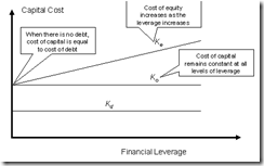
Figure 1. Capital cost according to NOI approach

If what is argued in this approach was to be completely applicable to the real practices of private equity firms, the attempt of increasing leverage would be meaningless. However there is one important point made clear with this approach is that the profit expectation of investors are getting higher with increased leverage. This is usually correct for common shareholders in listed companies. But as the private equity investors increase leverage, public equity contribution is getting less in the total capital and public equity investors’ concerns and their valuation is getting less important too. Therefore, even in the theoretical level, the assumption that capital cost remains constant even at higher leverage does not hold for this case.

Modigliani and Miller Approach

In 1958 Modigliani and Miller (M&M) presented their ground breaking study and changed all the perception of financial managers who are trying to maximise their companies’ value. They advocated that the relationship between financial leverage and the cost of capital is explained by the NOI approach and provide behavioural justification for a constant K_o over the entire range of financial leverage possibilities.

They argued they the value of the company is irrelevant of how its capital is financed through the combination of debt and equity. This argument was suggested under the assumption of a market where there is no corporate taxation. If a company is not liable to pay taxes, the value that it can generate trough equity is supposed to be the same as the value generated through debt. In other words, companies can use leverage as much as they want as it has no effect on company value.

However, it is obvious that taxes form important part of the liabilities that managers have to take into account. And in fact it is one of the most important parameter that affects the capital structure. Even if M&M’s contribution of irrelevance theory, financial managers’ main aim is still to maximize company value and minimize the cost of capital.

The biggest advantage of debt over equity is that taxes are paid after interest. A manager would prefer to pay interest for their capital funding rather than paying a tax which costs more. So, the leverage would be pushed as much as possible until the point that it starts posing a danger of risk for business. As the leverage is increased, lenders would be less willing to give loan and investors would be less likely to invest so both cost of debt and cost of equity will rise. Therefore the most efficient capital structure must be sought where cost of capital is minimum.

According to M&M it is pointless to try to find the minimum cost of capital; financial managers may change the level of leverage as they wanted. So there is no way for any kind of capital structure inefficiencies by the private equity firm’s leverage adjustments. In fact, financial managers may use the same level of leverage even without using private equity and have the same chance to increase the cash flow as a private equity firm would do. However it is not the case in the real world and there are loads of other concerns which need attention by financial managers to keep the leverage in industry levels.

The next approach is more successful at explaining managers’ attitudes against determining leverage levels.

And also sheds more light on why leverage level would significantly differ in a company when its stakes are bought by a private equity fund management firms.

Net Income Approach (NI) and Traditional Approach

According to this approach, the cost of debt and the cost of equity do not change with a change in the leverage ratio, which results in a decline in cost of capital as leverage increases. This can be explained by the following equation which is used for calculation of weighted average of cost of capital.

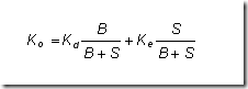
• K_o: average cost of capital
• K_d: cost of debt
• K_e: cost of equity
• B: market value of debt
• S: market value of equity

 

Figure 2. Capital cost according to NI approach

Since cost of debt is less than cost of equity and cost of debt gets higher weight against cost of equity as leverage increases; the average cost of capital decreases with the leverage. Figure 2 is the illustration of how weighted average of cost of capital changes with the leverage level.

Traditional approach is midway between the NI and the NOI approach. The main propositions of this approach are:

• The cost of debt remains almost constant up to a certain degree of leverage but rises thereafter at an increasing rate.
• The cost of equity remains more or less constant or rises gradually up to a certain degree of leverage and rises sharply thereafter.

The cost of capital due to the behaviour of the cost of debt and cost of equity

• Decreases up to a certain point
• Remains more or less constant for moderate increases in leverage thereafter
• Rises beyond that level at an increasing rate.

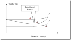
Figure 3. Capital cost according to traditional approach

As depicted in Figure 3, low-cost debt is not rising initially and replaces more expensive equity financing and K_o declines. Then, increasing financial leverage and the associated increase in K_e offsets the benefits of lower cost debt financing. Therefore according to this approach, cost of capital may hit a lowest point at a certain leverage level, where financial managers are trying to find. This is also the point where the firm’s total value will be the largest.

In a public company, finding optimum capital structure may be the one of the main aims for a financial manager. And the proposed theory presented above is closest to what is happening in practice. However when a public company chooses private equity to achieve its long term goals, the aim which is sought to maximise company value rather changes to realize potential growth, generate cash flow and satisfy private equity investors’ expectations.

The comparison between private equity and debt as a capital resource

Obtaining private equity is very different from raising debt or loan from a lender, such as a bank. Lenders have legal right to interest on a loan and repayment of the capital, irrespective of company’s success or failure.

Private equity backed companies have been shown to grow faster than other types of companies. This is made possible by the provision of a combination of capital and experienced personal input from private equity executives, which sets it apart from other forms of finance. Private equity can help companies to achieve their visions and provide a stable base for strategic decision making. Private equity firms will seek to increase company’s value to its owners, without taking day-to-day management control. Although the owners may have a smaller “slice of cake”, within a few years this “slice” should be worth considerably more than the whole “cake” was to them before.

Debt providers are secured with the interest payments and capital repayment of the loan. And these payments are usually guaranteed by business assets or company owners’ personal assets like home, land etc. If company defaults on its debt, as a last resort, lender has the right to ask liquation of any asset, which may lead bankruptcy. Therefore debt is secured in this way and has a higher priority than that of general unsecured creditors.

By contrast, private equity is not secured on any assets although part of the non-equity funding package provided by the private equity firm may seek some security. Therefore, private equity firm has the same risk of failure just like the other shareholders. Private equity firm is an equity business partner and is rewarded by the company’s success. This reward is usually achieved through realizing capital gain.

Private Equities

Private equities are equity securities of unquoted companies (companies that have not listed their stock on a public exchange). They provide long-term, committed share capital for firms and help them to grow and succeed. Private equity investors (also called financial sponsors or buy-out firms) typically hold their investments with the intent of realizing a return within 3 to 7 years. Generally, investments are realized through an initial public offering, sale, merger, or recapitalization.

Private equity is invested in exchange for a stake in company and the investors’ returns are dependent on the growth and profitability of the business. Private equity in the UK originated in the late 18th century, when entrepreneurs found wealthy individuals to back their projects. This informal method of financing became an industry in the late 1970s and early 1980s when a number of private equity firms were founded. Private equity is now a recognised asset class. There are over 170 active UK private equity firms, which provide several billion pounds each year to unquoted companies, around 80% of which are located in the UK (British Private Equity and Venture Capital Association, Aug 2007).

How does a private equity fund-management firm make money?

If an entrepreneur is looking to start up, expand, buy into a business, buy out a division of the parent company, turnaround or revitalise a company, private equity could help to do this.

The process typically involves a private equity fund-management firm raising a Limited Partnership fund, where private equity investors put money with limited liability. Investors usually cannot lose more than their capital contribution however they receive income, capital gains, and tax benefits. The fund is used to buy majority of stakes in business for long term. The equity fund-management firm will often look for an established and defendable market position with strong cash flow, a reasonable growth strategy and clear exit potential.

The new ownership structure can supply the company with risk capital to accelerate its growth, organically or by acquisition, or to restructure. The private market also shields a company from the demands of shareholders to deliver an instant payback on any investment.

The private equity manager actively helps the company to develop, normally by taking a seat on the board and providing strategic advice on capital markets and financing, market analysis, networking and sourcing other key executives. When the company has developed sufficiently to attract other investors, it may be sold to a larger company, floated on the stock market or sold to another private equity firm, which might be able to bring some other form of expertise to the party - surprisingly, 40% are sold on to other private equity firms (Moneywise, Aug 2007).

While venture capital firms tend to invest in earlier stage growth companies, private equity groups tend to focus on more mature businesses, often contributing both equity and debt (or some hybrid) to the transaction.

What do private equity firms look for in a potential acquisition?

• Strong management team.
• Ability to generate cash.
• Significant growth potential.
• Ability to create value.
• A clearly defined exit strategy.

Types of Investment Risk

In general terms investors who are in favour of risking their investments in pursuit of gaining more returns use equity type of securities. When there is a bull market, it is very hard for any other security to beat its profits. However there are also investors which prefer playing safe and therefore invest in fixed interest securities, broadly speaking bonds. Although it depends on how reliable is the issuer of bonds, investors gain lower but safer stream of income through them. Followings are main types of investment risks that an investor has to face.

Company Risk: (also known as unsystematic risk) company-specific events, such as a poor company reports at the end of the fiscal year, management change, legal action or the possibility of bankruptcy has an influence on stock prices.  Company risk is a concern for equity and corporate/high yield bond fund investors.

Country Risk:  This can be political, economic and other financial events which might have an influence over the value of foreign securities. Country risk is a potential concern for international bond and equity fund investors. 

Credit Risk:  The risk that the issuer of a security, such as a bond, may default on interest and/or principal payments or become bankrupt. Government bonds are usually regarded as higher quality bonds and face the lowest credit risk. By contrast, bonds that are issued by companies with poor credit ratings are subject to higher credit risk. Credit risk is a potential concern for bond fund investors. 

Currency Risk: The risk involved in transactions where more than one currency is involved. A movement in international exchange rates may change the cost of buying an asset before the purchase is completed. Currency risk is a potential concern for international equity bond fund investors.

Inflation Risk:  Inflation decreases the purchasing power of money so that it eliminates returns from an investment. Inflation risk is a potential concern for money market fund investors.

Interest Rate Risk: The risk that the value of a fixed income security will fluctuate as interest rates change. The value of a bond tends to move in the opposite direction of interest rates.  For instance, when interest rates rise the value of a bond will usually fall because it's stated coupon rate is lower than the going market rate.  Interest rate risk is a more immediate concern for bond fund investors.

Liquidity Risk: The risk that arises when a security cannot be sold easily.  Liquidity risk comes into play if an investment has to be sold quickly, but an insufficient secondary market prevents the liquidation of shares, or limits the price at which the security can be sold.  Liquidity risk is a potential concern for both bond and equity investors. 

Market Risk: (also known as systematic risk) The risk that applies to an entire asset class, with economic changes (e.g. recession) and other large events. An overall decline in the stock market may have a negative impact on the securities. Although the companies may be doing well, if there is a general decline in stock prices stock prices may decline in value anyway.

Investment Appraisal Techniques

Most businesses have a choice of a range of investment projects and they need to have a basis for comparing them to evaluate which is the best. Here are the most widely used methods for assessing candidate projects in terms of their return performances.

Payback period

The payback period is the simplest tools for appraising different investment projects. To be able to compare projects we need to have information on how much the project costs and the expected net cash flows or income streams that it is likely to generate over its lifetime. Following is an example to this method.

Let's say that a firm is planning to install a new computerized stock control system. The expected net cash flow (income less expenses) from the system is as follows and the expenses to be incurred for this system is £250,000.

Year	1	2	3	4	5
Net cash flow	50,000	65,000	65,000	70,000	75,000

We can see that the payback period on this system is exactly four years. This is because cumulative returns for the first 4 years of this project is equal to the cost of it. One can do this analysis in terms of months as well, if the figure does not come out as an exact number of years.

Average rate of return

The average rate of return, like the payback period method, looks at the expected net cash flows (income - expenses) of the investment project. It then measures the average net return each year as a percentage of the initial cost of the investment. Let's look at an example. A firm is looking at buying a new automatic painting machine. The cost of the machine is 200,000 and the expected net cash flows are:

Year	1	2	3	4	5
Net cash flow	50,000	55,000	65,000	75,000	75,000

The total return from the project over the five years is 320,000 (the sum of the five years). If we subtract the original cost of 200,000 from this, we get the net return from the investment to be 120,000. This took 5 years to earn and so the annual return is 120,000 divided by 5 which is 24,000 per annum. To get the average rate of return, we use the following formula:

Net return per annum Average rate of return = ---------------------- x 100                               Capital cost

From the figures above this gives us:

Average rate of return = 24,000 x 100 / 200,000 = 12%

This suggests that every £1 worth of investment yields an average 12p return each year

Discounted cash flow

Discounted cash flow (DCF) is the most realistic of the three methods, but has the main advantage that it takes account of the fact that returns in the future may be worth less than the same return now. As a result of this it may gives us far less amount of return than the other methods are projecting.

To use this to value an investment project, we would go through the following steps:

• Choose an estimated discount rates for the years that project is run (this may depend on expected future interest rates in the market).
• Find the present values by multiplying the expected net cash flows with their discount factor.
• Add together all the present values from step 2 and subtract the capital cost to give us the net present value.

Let's do an example to see how this works. A firm is thinking of buying a machine costing £200,000 and the expected net cash flows are:

Year	1	2	3	4	5
Net cash flow	50,000	55,000	65,000	75,000	75,000

If we follow the three steps above, we will get:

Step 1

Let's choose a discount rate of 10%. This means that our discount factors are:

Years in future	1	2	3	4	5
10%	0.909	0.826	0.751	0.683	0.621

Step 2

If we multiply the expected net cash flow by the discount factor, we get:

Year	1	2	3	4	5
Net cash flow	50,000	55,000	65,000	75,000	75,000
10%	0.909	0.826	0.751	0.683	0.621
Present value (£)	45,450	45,430	48,815	51,225	46,575

Step 3

If we add all these present values together and subtract the capital cost, we get:

£237,495 - £200,000 = Net present value of £37,495

This represents quite a small return of 18.7% (37,495/200,000) over 5 years on the original investment. The average rate of return calculation gives us a result of 12% per annum on these same figures and so discounting the future value of returns does give a very different picture.

References

1. http://www.bized.co.uk/virtual/bank/business/finance/investment/expl.htm

The Advantages of Accruals Accounting

As seen from the examples above the accrual accounting is more accurate in terms of assessing financial position of company since it matches income with the expenses incurred to produce it. It allows financial managers to measure company’s performance with more realistic figures. In cash accounting, financial statements may be showing positive cash flows even if company may be going broke because of the expenses which have been accrued but not yet paid. Therefore accrual accounting is much safer as a measurement tool over cash accounting.

As the complexity of business transactions increased, the need for more accurate financial information led the financial managers to move from cash accounting to accruals accounting.  The companies which sell their products and services on credits or have projects that provide cash flows not just for current period but over a long term have been struggling to see their financial position. The accruals accounting is able to overcome these problems by combining current and future cash flows in the same financial statements.

Accruals accounting also allows more effective comparisons against other financial institutions which are using same accounting principle or industry standards.

Apart from the timing differences of transaction recording, in the accruals reporting, followings are treated differently:

Superannuation

Superannuation is the pension, which companies or governments are liable to pay to employees upon their retirements. They are usually made through trust funds. Accruals accounting records superannuation liabilities whether they are funded or unfunded. Also the number of employees, assumptions on wages growth, inflation and expected rate of return on investments are taken into account while calculating changes in the stock of unfunded liabilities.

Depreciation

Accrual accounting records cost of capital investment across the life of asset as depreciation, whereas cash accounting records this capital expenditure in a given fiscal year.

Public Debt Interest PDI

Under cash accounting PDI is recorded as the interest paid during the year. Under an accrual approach, allowance is made for interest accrued, but not actually paid, during the period.

Taxation Revenue

When revenue is accrued at the time of economic transaction, company becomes liable to pay tax on this revenue whether it is earned or not. Therefore very consistent and reliable method for accrual estimations is needed. However it is very difficult to know when all such transactions occur. As a result, it’s been put into practice that the revenue is only recognized as accruing when the relevant law indicates the existence of requirement or the taxpayer makes a self assessment.

The advantages of accruals accounting can be summarised as below:

• Improved accountability and better financial management.
• Reflects full scope of company’s resources (all assets), obligations (all liabilities) and costs (resources consumed).
• Provides more focus on the business output rather than input.
• Helps financial managers to use company resources more efficiently.
• Establishes a better link of resources and results yielded from these resources.
• Full cost of product or services can be compared across industry standards.

Differences Between Cash Accounting and Accruals Accounting

There are two main methods of accounting used in the business: cash accounting and accruals accounting. The basic difference is the timing of income and expense recording. The choice of the method depends on the factors like the nature of the business, ease of use or regulations by the related laws.

In cash accounting income is recognized when cash is received or deposited and expenses are recorded when bills are paid. Therefore transactions are recorded only when cash is handed over. Consequently non-cash transactions are excluded (such as provisions and revaluations).

In accruals accounting, economic events are recognized by matching revenues to expenses (the matching principle) at the time in which the transaction occurs rather than when payment is made (or received). Therefore accruals accounting measures the performance and position of a company by combining current cash flows with future expected cash flows, giving a more accurate picture of current financial condition.

The accruals concept and matching principle can be illustrated simply with the following example. Suppose a business had the following transaction at given times:

• Company purchases goods costing £100 on credit on 15 January.
• Bills are paid on 15 February for the goods purchased on 15 January.
• These goods are sold on credit for £150 on 15 March.
• On the 15 April Company receives payment for the goods sold on 15 March.

In the accruals accounting transactions are recognized in the following months:

1. The cost of goods is incurred in January.
2. The sales revenue is earned in March.
3. There is no profit or loss in January, February or April.

The only profit was earned in March which was £50 in total. The cost of goods is recorded as stock at the end of January and February.

As opposed to the accrual method, cash accounting would record same transactions in the following months:

1. The cost of goods is incurred in February.
2. The sales revenue is earned in April.
3. The profit is earned in April.

Accruals accounting is perceived as the standard practice in the business. Only in the certain cases, the small companies still may prefer cash accounting as they are less likely to operate on credits. Accrual method provides more accurate picture of company’s current financial condition and their financial statements are relatively more detailed. Accrual basis balance sheets have more items to be listed as they record non cash transactions.

Following is an illustration of differences between cash basis and accrual basis financial statements. Take an example of a weekend school operating on donations. At the end of the fiscal year, school has recorded its transactions based on its check book to produce cash basis income statement and balance sheet:

Cash basis statements

Income statement as at 31 December 2006
Income
Grants	£3.000
Contributions	£4.500
Fees from students	£25.000
Total Income	£32.500
Expenses
Salaries	£20,000
Food and supplies	£6.000
Insurance	£4.250
Utilities	£2.000
Telephone	£750
Printing and postage	£3.500
Total expenses	£36.450

 

Balance Sheet as at 31 December 2006
Fixed assets
Property and equipment	£120,000
Accumulated depreciation	<£100,000>
Current assets
Cash	£2.500
Less: Current Liabilities
Loan from founder	£10,000
Net current assets	£12. 500

All these activities have been taken from the check book, so these statements were produced on cash basis. This results in some of the pertinent information missing from the statements. Such as:

• Local government authorities had given a grant of £15.000 to provide scholarship for low-income students.
• There have been some students who attended school during last academic year and paid their fees in check, which has not been yet cashed. And this amounts £3.000 in total.
• The school management did not pay the final installment for some of the goods that they bought last year. They still owe £2.000 to the creditors.
• Company has already paid its insurance for the next 3 months in advance to the date of this statement is made. Therefore we can deduct (4250/12) x 3 = 1.062 from the insurance item.

If we want to take these factors into account all transactions need to be recorded on accrual basis. In order to do this we’ll add new items to financial statements and reproduce it on accrual basis. Followings are accrual basis statements of this weekend school for the same fiscal year.

Accrual basis statements

Income statement as at 31 December 2006
Income
Grants	£18.000
Contributions	£4.500
Fees from students	£28.000
Total Income	£50.500
Expenses
Salaries	£20,000
Food and supplies	£6.000
Insurance	£3.188
Utilities	£2.000
Telephone	£750
Printing and postage	£5.500
Total expenses	£37.438

 

Balance Sheet as at 31 December 2006
Fixed assets
Property and equipment	£120,000
Accumulated depreciation	<£100,000>
Current assets
Cash	£2.500
Accounts Receivable	£18.000
Prepaid Expenses	£1.062
Less: Current Liabilities
Loan from founder	£10,000
Accounts Payable	£2.000
Net current assets	£29.562

We have added three more items to reflect accruals on the balance sheet. These are “accounts receivables” for the transactions which have not yet received, “prepaid expenses” which have already paid and “accounts payable” for the items which company is liable to pay.

It is obvious that, accruals accounting requires more work to collect data and more resources are needed other than check book. We can say that cash accounting is much easier in terms of populating data and to produce financial statements. This is why still some of the small companies prefer to use cash accounting.
The very obvious reasons for choosing cash accounting can be summarized as follows:

1. Cash accounting principles are easier to understand than that of the accrual accounting principles.
2. Considering the costs involved in hiring accountants for accrual accounting, cash accounting seems to be cheaper.
3. In terms of tax planning, cash accounting is more attractive since the company is taxed on its current cash flow, not from the accounts receivables.

Given these advantages there are still companies which might see cash accounting more attractive for their business. However accrual accounting is now regarded as a industry standards and also not all companies has the freedom of choosing any accounting method since it is controlled by the governmental authorities.